Biostat 823 - Literate Programming

Hilmar Lapp

Duke University, Department of Biostatistics & Bioinformatics

2024-08-29

Literate Programming

  • First introduced by Donald Knuth (“The Art of Computer Programming”) in 1984

    Let us change our traditional attitude to the construction of programs: Instead of imagining that our main task is to instruct a computer what to do, let us concentrate rather on explaining to human beings what we want a computer to do.

    D. E. Knuth, Literate Programming, The Computer Journal, Volume 27, Issue 2, 1984, Pages 97–111, https://doi.org/10.1093/comjnl/27.2.97

TANGLE and WEAVE

Figure 1 from Knuth (1984)

Lit. Prog. and Reproducible Research

Literate Programming: Enhances traditional software development by embedding code in explanatory essays and encourages treating the act of development as one of communication with future maintainers

Reproducible Research: Embeds executable code in research reports and publications, with the aim of allowing readers to re-run the analyses described.

Code not paper is the scholarship

An article about computational science in a scientific publication is not the scholarship itself, it is merely advertising of the scholarship. The actual scholarship is the complete software development environment and complete set of instructions which generated the figures.

Research Compendium

  • Encapsulates the actual work, not just an abridged version;
  • Allows different levels of detail in different renderings;
  • Easy to re-run by anyone;
  • Provides explicit computational details, enabling others to adapt and extend the reported computational methods;
  • Enables programmatic construction and clear provenance of plots and tables;

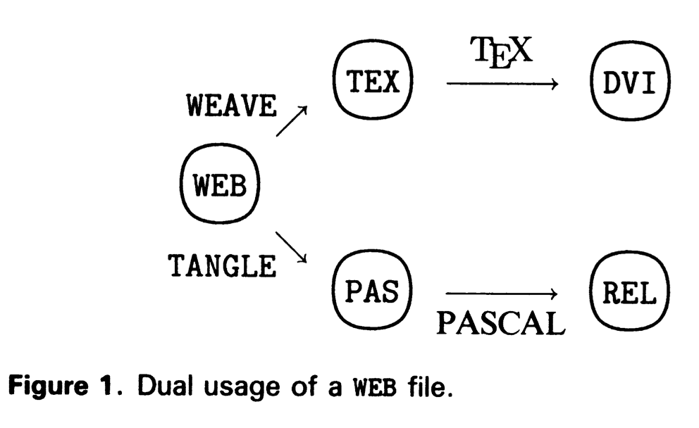
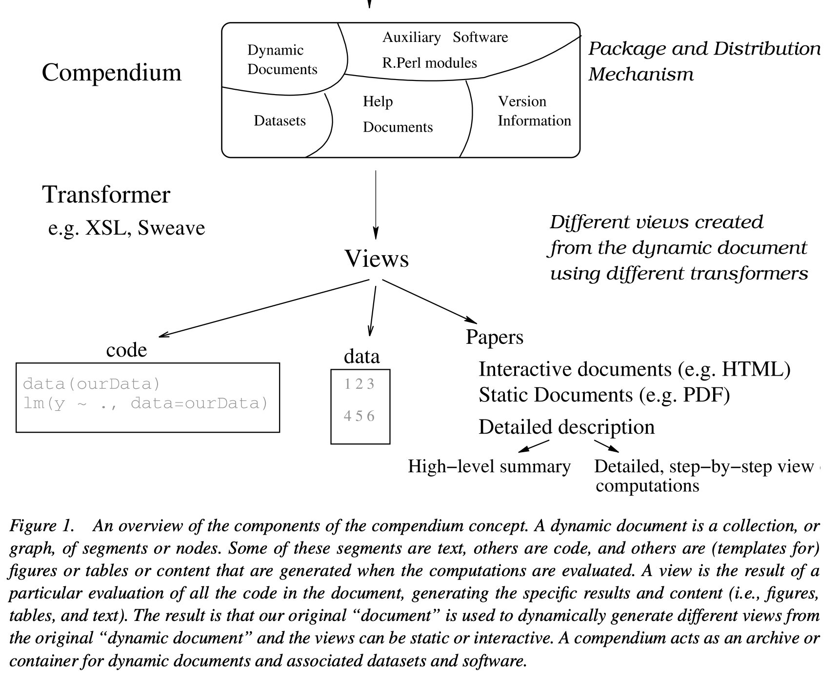
Part of Figure 1, Gentleman and Temple Lang (2007)

Reproducible research lens

Embeds executable code in research reports and publications, with the aim of allowing readers to re-run the analyses described. (Schulte et al (2012))

Important concepts:

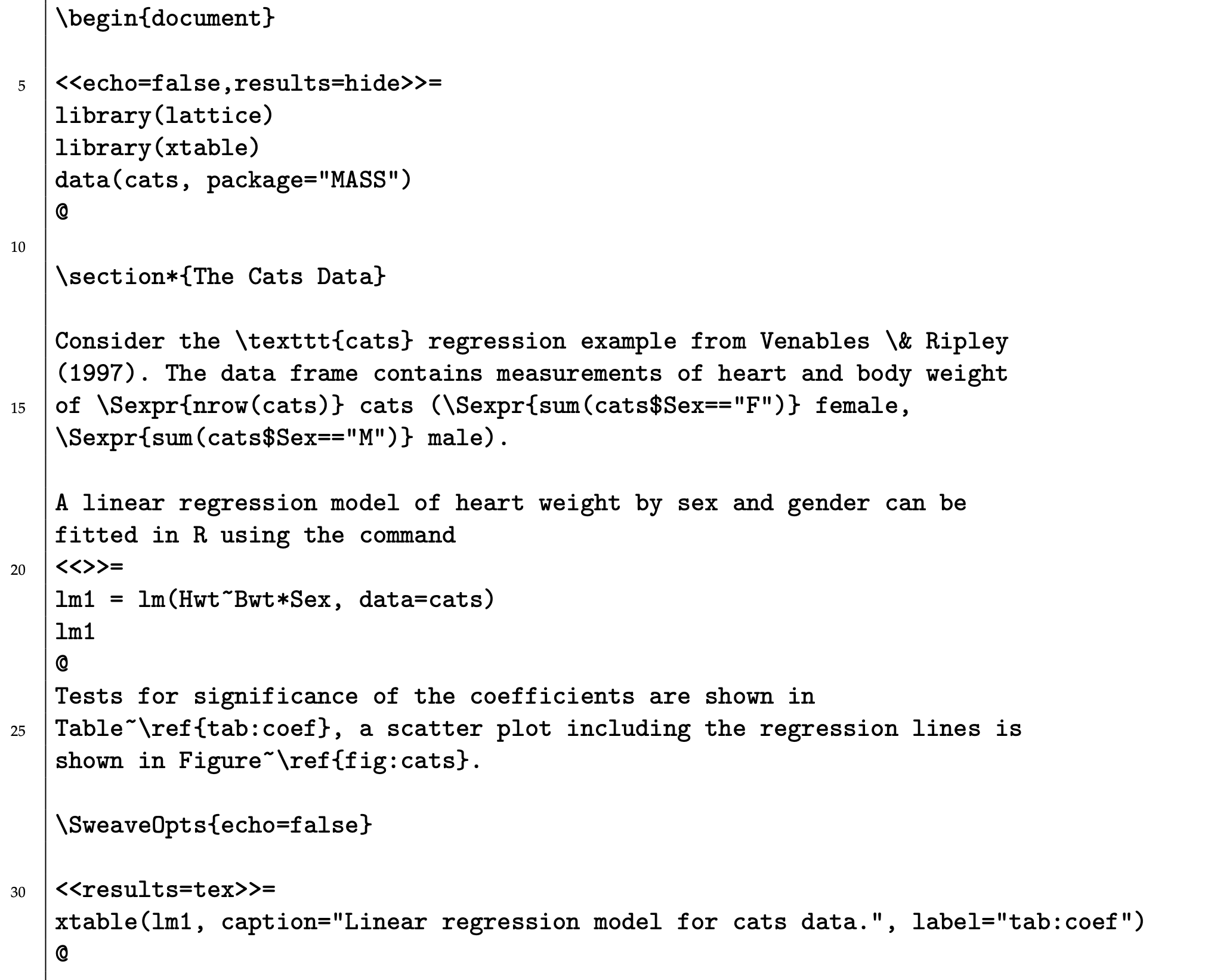
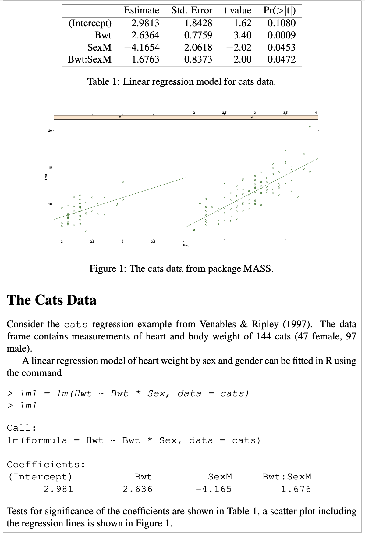
  • Ties together narrative (the “why”), code that implements it, and the results from running the code.
  • Can be executed (“executable paper”), in its original or modified form.
  • Provenance of tables and charts is clear and verifiable.

Sweave (Leisch 2002)

Part of Figure 1, F. Leisch (2002). “Sweave, Part I: Mixing R and LaTeX: A short introduction to the Sweave file format and corresponding R functions”. R News. 2 (3): 28–31.

Figure 2, F. Leisch (2002)

Renewed interest for reproducible computing

  • The practice of copying values for tables and plots for figures into a document breaks the provenance chain.

Provenance: Information about entities, activities, and people involved in producing data or other results, which are necessary to assess their quality, reliability or trustworthiness.1

“Executable Paper” concept:

Jupyter and iPython Notebooks

Knitr and Rmarkdown

  • Knitr created by Yihui Xie, first released 2012
    • Designed as a general-purpose literate programming engine
    • Design allows different input languages and different output formats
  • Rmarkdown
    • First introduced in knitr in early 2012, withh the idea to embed code chunks in Markdown documents.
    • rmarkdown R package created in 2014
    • Rich universe of examples at RPubs

Markdown and code

In Rmarkdown, code can be inline:

Consider Edgar Anderson's Iris data of sepal and petal lengths measurements
of `r nrow(iris)` flowers, (`r sum(iris$Species=="setosa")` _I. setosa_,
`r sum(iris$Species=="versicolor")` _I. versicolor_, and
`r sum(iris$Species=="virginica")` _I. virginica_).

Consider Edgar Anderson’s Iris data of sepal and petal lengths measurement of 150 flowers, (50 I. setosa, 50 I. versicolor, and 50 I. virginica).

Code chunks

A linear regression model of petal width by sepal length can be fitted in the following way:

```{r}
lm1 = lm(Petal.Width ~ Sepal.Length, data=iris)
summary(lm1)
```

Rendered:

lm1 = lm(Petal.Width ~ Sepal.Length, data=iris)
summary(lm1)

Call:
lm(formula = Petal.Width ~ Sepal.Length, data = iris)

Residuals:
     Min       1Q   Median       3Q      Max 
-0.96671 -0.35936 -0.01787  0.28388  1.23329 

Coefficients:
             Estimate Std. Error t value Pr(>|t|)    
(Intercept)  -3.20022    0.25689  -12.46   <2e-16 ***
Sepal.Length  0.75292    0.04353   17.30   <2e-16 ***
---
Signif. codes:  0 '***' 0.001 '**' 0.01 '*' 0.05 '.' 0.1 ' ' 1

Residual standard error: 0.44 on 148 degrees of freedom
Multiple R-squared:  0.669, Adjusted R-squared:  0.6668 
F-statistic: 299.2 on 1 and 148 DF,  p-value: < 2.2e-16

Plots also get inlined

Plots of the regression residuals etc can be obtained in the following way:

plot(lm1)

Ecosystem

One report document, rendered to many different output formats

Further reading